

Bob’s Imaging Fundamentals #12: Graphs Part 1
An Image Processing Perspective
My earliest memories of graphs take me back to ‘grade whatever’, when I was first introduced to the Cartesian-X/Y torture device. I remember looking up, having finished my first, beautiful X/Y axes, only to realize I had completely missed the explanation of what to do next. My relationship with graphs went downhill from there.
Today though, thanks to machine vision and image processing, graphs are my friend. One of the cool things about graphs is you can make the X/Y axes represent whatever you want. For instance, let’s make the Y-axis a pixel’s value (i.e. a monochrome image will have a range of 0 to 255) and we’ll make the X-axis represent the pixel’s horizontal position in the image. Now, if we take a look at line 43 in our picture Doraimon, and we plot the value of each pixel on our graph, we end up with a nifty profile of each pixel’s value along line 43:
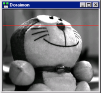
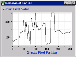
Essentially, this graph shows us the nature and magnitude of the changes in pixel values along the red line (line 43). Line (and/or column) profile information can sometimes be useful when trying to find clues to help solve a machine vision problem. For instance, looking at line 43’s profile around the 150 position, shows us that there is a huge jump from dark to light pixel values, when we go from Doraimon’s nose to the bottom of his eye. Is this information useful? Maybe, maybe not, it all depends on the approach you decide to take in solving your particular machine vision problem.
Next time, we’re going to try to make a graph jump through a hoop! Back Simba! Back!